文章

代数拓扑中的微分形式

作者：Pleut

发布于 2026-07-12T06:42:39Z · 公开内容更新于 2026-08-17T13:53:33Z

代数拓扑中的微分形式 pleut (August 10, 2026) 参考：GTM82及Loring W Tu于台湾大学的课程（录像公开在台大官网） Chapter De Rham Cohomology 1 Tensors and Forms 1.1 Tensors definition [ 𝑘 -tensor] A

代数拓扑中的微分形式

pleut

(October 8, 2026)

参考：GTM82及Loring W Tu于台湾大学的课程（录像公开在台大官网）

1 De Rham Cohomology

1.1 Tensors and Forms

1.1.1 Tensors

Definition 1.0.1 ( $𝑘$ -tensor).

A $𝑘$ -tensor on a vector space $𝑉$ is a $𝑘$ -linear function

𝑉 \times \dots \times 𝑉 ⏟__⏟__⏟ 𝑘 t i m e s ⟶ ℝ .

Example 1.0.1 ( Dual Space).

The dual space of a vector space $𝑉$ is

𝑉 \lor = {𝑓 : 𝑉 \to ℝ ∣ 𝑓 i s l i n e a r} .

Elements of $𝑉 \lor$ are precisely 1-tensors on $𝑉$ .

Definition 1.0.2 (Alternating $𝑘$ -tensor).

A $𝑘$ -tensor $𝛼$ is alternating if for any permutation $𝜎 \in 𝑆 𝑘$ ,

𝛼 (𝑉 𝜎 (1), \dots, 𝑉 𝜎 (𝑘)) = s g n (𝜎) 𝛼 (𝑉 1, \dots, 𝑉 𝑘) .

We denote by $𝐴 𝑘 (𝑉)$ the space of alternating $𝑘$ -tensors on $𝑉$ .

Remark 1.0.1.

1.

Elements of $𝑉 \lor$ are automatically alternating, i.e. $𝑉 \lor = 𝐴 1 (𝑉)$
2.

The k-tensor and alternating k-tensor form two vector spaces, the vector space formed by alternating k-tensor is a subspace of k-tensor’s.

Example 1.0.2.

For $𝑉 = ℝ 3$ , the determinant $d e t (𝑎, 𝑏, 𝑐)$ for $𝑎, 𝑏, 𝑐 \in ℝ 3$ is a 3-linear alternating tensor.

Definition 1.0.3 (Wedge Product).

If $𝛼 \in 𝐴 𝑘 (𝑉)$ and $𝛽 \in 𝐴 𝑙 (𝑉)$ , then $𝛼 \land 𝛽 \in 𝐴 𝑘 + 𝑙 (𝑉)$ is defined by

(𝛼 \land 𝛽) (𝑉 1, \dots, 𝑉 𝑘 + 𝑙) = 1 𝑘! 𝑙! \sum 𝜎 \in 𝑆 𝑘 + 𝑙 s g n (𝜎) 𝛼 (𝑉 𝜎 (1), \dots, 𝑉 𝜎 (𝑘)) 𝛽 (𝑉 𝜎 (𝑘 + 1), \dots, 𝑉 𝜎 (𝑘 + 𝑙)) .

Example 1.0.3.

If $𝛼, 𝛽 \in 𝐴 1 (𝑉)$ , then

(𝛼 \land 𝛽) (𝑉 1, 𝑉 2) = 𝛼 (𝑉 1) 𝛽 (𝑉 2) - 𝛼 (𝑉 2) 𝛽 (𝑉 1) .

Proposition 1.0.1 (Basis of Alternating Tensors).

If ${𝑎 1, \dots, 𝑎 𝑛}$ is a basis for $𝑉 \lor$ , then

{𝑎 𝑖 1 \land \dots \land 𝑎 𝑖 𝑘 ∣ 1 \leq 𝑖 1 < \dots < 𝑖 𝑘 \leq 𝑛}

is a basis for $𝐴 𝑘 (𝑉)$ .

Let $𝑈$ be an open subset of $ℝ 𝑛$ , and let $𝑝 \in 𝑈$ . The tangent space at $𝑝$ is

𝑇 𝑝 𝑈 ≅ ℝ 𝑛,

with basis ${𝜕 𝜕 𝑥 1 ∣ 𝑝, \dots, 𝜕 𝜕 𝑥 𝑛 ∣ 𝑝}$ .

1.1.2 Differential Forms

Definition 1.0.4 (Differential Form).

A $𝑘$ -form on $𝑈$ is an assignment to each point $𝑝 \in 𝑈$ of an alternating $𝑘$ -tensor

𝜔 𝑝 : 𝑇 𝑝 𝑈 \times \dots \times 𝑇 𝑝 𝑈 ⏟___⏟___⏟ 𝑘 t i m e s ⟶ ℝ .

Equivalently, a $𝑘$ -form is a function

𝜔 : 𝑈 ⟶ ⋃ 𝑝 \in 𝑈 𝐴 𝑘 (𝑇 𝑝 𝑈) .

Remark 1.0.2.

k-form forms a vector space.

Definition 1.0.5 (Differential of a Function).

For $𝑓 \in 𝐶 \infty (𝑈)$ , define the 1-form $𝑑 𝑓$ by

(𝑑 𝑓) 𝑝 (𝑣) = 𝑣 𝑓 = 𝑛 \sum 𝑖 = 1 𝑣 𝑖 𝜕 𝑓 𝜕 𝑥 𝑖 (𝑝),

where $𝑣 = \sum 𝑣 𝑖 𝜕 𝜕 𝑥 𝑖 ∣ 𝑝 \in 𝑇 𝑝 𝑈$ .

The $𝑥 𝑖$ can be viewed as a function, which gives the i-th coordinate.
Then for each $𝑖 = 1, \dots, 𝑛$ , the 1-form $𝑑 𝑥 𝑖$ , by definition

(𝑑 𝑥 𝑖) 𝑝 (𝜕 𝜕 𝑥 𝑗 ∣ 𝑝) = 𝛿 𝑖 𝑗 .

(𝑑 𝑥 𝑖) 𝑝 (𝑣) = 𝑣 𝑥 𝑖 = 𝑛 \sum 𝑗 = 1 𝑣 𝑗 𝜕 𝑓 𝜕 𝑥 𝑗 (𝑥 𝑖) = 𝑣 𝑖

Thus $𝑑 𝑥 𝑖$ picks out the $𝑖$ -th coordinate of a tangent vector.

Proposition 1.0.2 ( The expression of k-form in the local coordinate).

Every $𝑘$ -form $𝜔$ on $𝑈$ can be written uniquely as

𝜔 = \sum 𝑖 1 < \dots < 𝑖 𝑘 𝑎 𝑖 1 \dots 𝑖 𝑘 𝑑 𝑥 𝑖 1 \land \dots \land 𝑑 𝑥 𝑖 𝑘 = : \sum 𝐼 𝑎 𝐼 𝑑 𝑥 𝐼,

where $𝐼 = (𝑖 1, \dots, 𝑖 𝑘)$ with $1 \leq 𝑖 1 < \dots < 𝑖 𝑘 \leq 𝑛$ .

Definition 1.0.6 (Smooth Forms).

A $𝑘$ -form $𝜔 = \sum 𝐼 𝑎 𝐼 𝑑 𝑥 𝐼$ is smooth (or $𝐶 \infty$ ) if all coefficient functions $𝑎 𝐼$ are $𝐶 \infty$ . We denote

Ω 𝑘 (𝑈) = {𝐶 \infty 𝑘 - f o r m s o n 𝑈} .

Theorem 1.1 (Exterior Derivative).

There exists a unique $ℝ$ -linear map

𝑑 : Ω 𝑘 (𝑈) ⟶ Ω 𝑘 + 1 (𝑈)

satisfying:

1.

$𝑑$ is an antiderivation:

$𝑑 (𝜔 \land 𝜏) = 𝑑 𝜔 \land 𝜏 + (- 1) 𝑘 𝜔 \land 𝑑 𝜏, 𝜔 \in Ω 𝑘 (𝑈) .$
2.

$𝑑 \circ 𝑑 = 0$ , i.e. $𝑑 2 = 0$ .
3.

On $Ω 0 (𝑈) = 𝐶 \infty (𝑈)$ , $𝑑$ is the usual differential: $𝑑 𝑓 = \sum 𝑖 𝜕 𝑓 𝜕 𝑥 𝑖 𝑑 𝑥 𝑖$ .

Remark 1.1.1.

For a $𝑘$ -form $𝜔 = \sum 𝐼 𝑎 𝐼 𝑑 𝑥 𝐼$ , the exterior derivative is given by

𝑑 𝜔 = \sum 𝐼 𝑑 𝑎 𝐼 \land 𝑑 𝑥 𝐼 = \sum 𝐼 𝑛 \sum 𝑗 = 1 𝜕 𝑎 𝐼 𝜕 𝑥 𝑗 𝑑 𝑥 𝑗 \land 𝑑 𝑥 𝐼 .

Let $𝑈 \subseteq ℝ 𝑛$ be open. The sequence

0 ⟶ Ω 0 (𝑈) 𝑑 0 ⟶ Ω 1 (𝑈) 𝑑 1 ⟶ \dots 𝑑 𝑛 - 1 \leftarrow\leftarrow\leftarrow\leftarrow\leftarrow\leftarrow\leftarrow \to Ω 𝑛 (𝑈) ⟶ 0

is called the de Rham complex of $𝑈$ . Since $𝑑 𝑘 \circ 𝑑 𝑘 - 1 = 0$ , we have

I m 𝑑 𝑘 - 1 \subseteq k e r 𝑑 𝑘 .

Definition 1.1.1 (Closed and Exact Forms).

•

A $𝑘$ -form $𝜔 \in Ω 𝑘 (𝑈)$ is closed if $𝑑 𝜔 = 0$ . The space of closed $𝑘$ -forms is denoted

$𝑍 𝑘 (𝑈) = k e r 𝑑 𝑘 .$
•

A $𝑘$ -form $𝜔 \in Ω 𝑘 (𝑈)$ is exact if $𝜔 = 𝑑 𝜂$ for some $𝜂 \in Ω 𝑘 - 1 (𝑈)$ . The space of exact $𝑘$ -forms is denoted

$𝐵 𝑘 (𝑈) = I m 𝑑 𝑘 - 1 .$

1.2 The De Rham Cohomology

1.2.1 De Rham Cohomology

Definition 1.1.2 (De Rham Cohomology).

The $𝑘$ -th de Rham cohomology of $𝑈$ is the quotient vector space

𝐻 𝑘 (𝑈) = k e r 𝑑 𝑘 I m 𝑑 𝑘 - 1 = 𝑍 𝑘 (𝑈) 𝐵 𝑘 (𝑈) .

Example 1.1.1 ( Computation of $𝐻 * (ℝ)$ ).

Consider the de Rham complex for $𝑈 = ℝ$ :

0 ⟶ Ω 0 (ℝ) 𝑑 0 ⟶ Ω 1 (ℝ) ⟶ 0 .

Computation of $𝐻 0 (ℝ)$

𝑍 0 (ℝ) = {𝑓 \in 𝐶 \infty (ℝ) ∣ 𝑑 𝑓 = 0} .

Since $𝑑 𝑓 = 𝑓' (𝑥) 𝑑 𝑥$ , we have $𝑑 𝑓 = 0 ⟺ 𝑓' (𝑥) = 0 ⟺ 𝑓 i s c o n s t a n t$ . Thus

𝑍 0 (ℝ) ≅ ℝ .

Also,

𝐵 0 (ℝ) = I m 𝑑 - 1 = 0 .

Therefore,

𝐻 0 (ℝ) = 𝑍 0 (ℝ) / 𝐵 0 (ℝ) ≅ ℝ .

Computation of $𝐻 1 (ℝ)$

𝑍 1 (ℝ) = {𝑔 (𝑥) 𝑑 𝑥 ∣ 𝑑 (𝑔 (𝑥) 𝑑 𝑥) = 0} .

But $𝑑 (𝑔 (𝑥) 𝑑 𝑥) = 0$ automatically, so

𝑍 1 (ℝ) = {𝑔 (𝑥) 𝑑 𝑥 ∣ 𝑔 \in 𝐶 \infty (ℝ)} ≅ 𝐶 \infty (ℝ) .

Next,

𝐵 1 (ℝ) = {𝑑 𝑓 ∣ 𝑓 \in 𝐶 \infty (ℝ)} = {𝑓' (𝑥) 𝑑 𝑥 ∣ 𝑓 \in 𝐶 \infty (ℝ)} .

Given any $𝑔 \in 𝐶 \infty (ℝ)$ , define

𝑓 (𝑥) = \int 𝑥 0 𝑔 (𝑡) 𝑑 𝑡 .

Then $𝑓 \in 𝐶 \infty (ℝ)$ and $𝑓' (𝑥) = 𝑔 (𝑥)$ . Hence $𝑔 (𝑥) 𝑑 𝑥 = 𝑑 𝑓$ , so

𝑍 1 (ℝ) = 𝐵 1 (ℝ) .

Therefore,

𝐻 1 (ℝ) = 0 .

Proposition 1.1.1.

The de Rham cohomology of $ℝ$ is

𝐻 𝑘 (ℝ) = {ℝ, 𝑘 = 0, 0, 𝑘 \geq 1 .

1.2.2 Cohomology with Compact Support

Definition 1.1.3 (Support of a Differential Form).

Let $𝑈 \subseteq ℝ 𝑛$ be open, and let $𝜔 \in Ω 𝑘 (𝑈)$ be a $𝑘$ -form. The zero set of $𝜔$ is defined as

𝑍 (𝜔) = {𝑝 \in 𝑈 ∣ 𝜔 𝑝 = 0} .

The support of $𝜔$ is the closure in $𝑈$ of the complement of the zero set:

s u p p 𝜔 = c l 𝑈 (𝑈 ∖ 𝑍 (𝜔)) = c l 𝑈 (𝑍 (𝜔) 𝑐) .

In other words, the support of $𝜔$ is the smallest closed set outside which $𝜔$ is identically zero.

Definition 1.1.4 (Compact Support Forms).

Let $𝑈 \subseteq ℝ 𝑛$ be open. We denote by

Ω 𝑘 𝑐 (𝑈) = {𝜔 \in Ω 𝑘 (𝑈) ∣ s u p p 𝜔 i s c o m p a c t i n 𝑈}

the space of smooth $𝑘$ -forms with compact support.

Proposition 1.1.2 (Support is Decreasing under $𝑑$ ).

For any $𝜔 \in Ω 𝑘 𝑐 (𝑈)$ , we have

s u p p (𝑑 𝜔) \subseteq s u p p 𝜔 .

In particular, if $𝜔$ has compact support, then so does $𝑑 𝜔$ .

Proof.

We prove the equivalent statement

(s u p p 𝜔) 𝑐 \subseteq (s u p p 𝑑 𝜔) 𝑐 .

Let $𝑝 \in (s u p p 𝜔) 𝑐$ . Since $s u p p 𝜔$ is closed, there exists an open neighbourhood $𝑉 \subseteq 𝑈$ of $𝑝$ such that

𝑉 \subseteq 𝑈 ∖ s u p p 𝜔 .

Hence $𝜔 \equiv 0$ on $𝑉$ . Therefore, $𝑑 𝜔 \equiv 0$ on $𝑉$ , which means

𝑝 \notin s u p p (𝑑 𝜔) .

Thus $𝑝 \in (s u p p 𝑑 𝜔) 𝑐$ , proving the inclusion. Consequently,

s u p p (𝑑 𝜔) \subseteq s u p p 𝜔 .

Since $s u p p 𝜔$ is compact and $s u p p (𝑑 𝜔)$ is closed, it follows that $s u p p (𝑑 𝜔)$ is also compact. Hence $𝑑 𝜔 \in Ω 𝑘 + 1 𝑐 (𝑈)$ . ∎

Corollary 1.1.1.

The exterior derivative restricts to a linear map

𝑑 : Ω 𝑘 𝑐 (𝑈) ⟶ Ω 𝑘 + 1 𝑐 (𝑈) .

Thus the sequence

0 ⟶ Ω 0 𝑐 (𝑈) 𝑑 \to Ω 1 𝑐 (𝑈) 𝑑 \to \dots 𝑑 \to Ω 𝑛 𝑐 (𝑈) ⟶ 0

is a cochain complex, called the de Rham complex with compact support.

Definition 1.1.5 (Compact Support Cohomology).

The $𝑘$ -th de Rham cohomology with compact support of $𝑈$ is the quotient

𝐻 𝑘 𝑐 (𝑈) = 𝑍 𝑘 𝑐 (𝑈) 𝐵 𝑘 𝑐 (𝑈),

where

𝑍 𝑘 𝑐 (𝑈) = k e r (𝑑 : Ω 𝑘 𝑐 (𝑈) \to Ω 𝑘 + 1 𝑐 (𝑈))

is the space of closed compactly supported $𝑘$ -forms, and

𝐵 𝑘 𝑐 (𝑈) = I m (𝑑 : Ω 𝑘 - 1 𝑐 (𝑈) \to Ω 𝑘 𝑐 (𝑈))

is the space of exact compactly supported $𝑘$ -forms.

Example 1.1.2 ( $𝐻 * 𝑐 (ℝ)$ ).

Let us compute the compact support cohomology of $ℝ$ . The complex is

0 ⟶ Ω 0 𝑐 (ℝ) 𝑑 \to Ω 1 𝑐 (ℝ) ⟶ 0 .

Computation of $𝐻 0 𝑐 (ℝ)$ : We have

𝑍 0 𝑐 (ℝ) = {𝑓 \in 𝐶 \infty 𝑐 (ℝ) ∣ 𝑑 𝑓 = 0} .

Since $𝑑 𝑓 = 𝑓' (𝑥) 𝑑 𝑥$ , the condition $𝑑 𝑓 = 0$ implies $𝑓' (𝑥) = 0$ , so $𝑓$ is constant. But a compactly supported constant function on $ℝ$ must be zero. Hence

𝑍 0 𝑐 (ℝ) = 0 .

Therefore,

𝐻 0 𝑐 (ℝ) = 0 .

Computation of $𝐻 1 𝑐 (ℝ)$ : First,

𝑍 1 𝑐 (ℝ) = {𝑔 (𝑥) 𝑑 𝑥 ∣ 𝑔 \in 𝐶 \infty 𝑐 (ℝ)},

since every 1-form on $ℝ$ is automatically closed. Also,

𝐵 1 𝑐 (ℝ) = {𝑑 𝑓 ∣ 𝑓 \in 𝐶 \infty 𝑐 (ℝ)} = {𝑓' (𝑥) 𝑑 𝑥 ∣ 𝑓 \in 𝐶 \infty 𝑐 (ℝ)} .

We claim that a compactly supported function $𝑔 \in 𝐶 \infty 𝑐 (ℝ)$ lies in $𝐵 1 𝑐 (ℝ)$ if and only if

\int + \infty - \infty 𝑔 (𝑥) 𝑑 𝑥 = 0 .

Indeed, if $𝑔 = 𝑓'$ for some $𝑓 \in 𝐶 \infty 𝑐 (ℝ)$ , then by the fundamental theorem of calculus,

\int + \infty - \infty 𝑔 (𝑥) 𝑑 𝑥 = \int + \infty - \infty 𝑓' (𝑥) 𝑑 𝑥 = 𝑓 (+ \infty) - 𝑓 (- \infty) = 0 .

Conversely, suppose $𝑔 \in 𝐶 \infty 𝑐 (ℝ)$ satisfies $\int + \infty - \infty 𝑔 (𝑥) 𝑑 𝑥 = 0$ . Define

𝑓 (𝑥) = \int 𝑥 - \infty 𝑔 (𝑡) 𝑑 𝑡 .

Then $𝑓' (𝑥) = 𝑔 (𝑥)$ . Moreover, for $𝑥$ sufficiently large (outside the support of $𝑔$ ), we have $𝑓 (𝑥) = \int + \infty - \infty 𝑔 (𝑡) 𝑑 𝑡 = 0$ , so $𝑓$ has compact support. Hence $𝑔 \in 𝐵 1 𝑐 (ℝ)$ .

Thus we have an exact sequence

0 ⟶ 𝐵 1 𝑐 (ℝ) ⟶ 𝑍 1 𝑐 (ℝ) \int + \infty - \infty \leftarrow\leftarrow\leftarrow\leftarrow\leftarrow\leftarrow\leftarrow\leftarrow\leftarrow \to ℝ ⟶ 0,

where the map is integration of the coefficient function. Therefore,

𝐻 1 𝑐 (ℝ) = 𝑍 1 𝑐 (ℝ) 𝐵 1 𝑐 (ℝ) ≅ ℝ .

In summary,

𝐻 𝑘 𝑐 (ℝ) = {0, 𝑘 = 0, ℝ, 𝑘 = 1 .

Remark 1.1.2.

Compare this with the ordinary de Rham cohomology of $ℝ$ :

𝐻 𝑘 (ℝ) = {ℝ, 𝑘 = 0, 0, 𝑘 \geq 1 .

The two cohomology theories differ significantly: compact support cohomology “detects” the non-compactness of $ℝ$ in degree 1, whereas ordinary cohomology detects it in degree 0.

1.3 Diffeomorphism Invariance

1.3.1 Pullback

Definition 1.1.6 (Pullback).

Let $𝐹 : 𝑀 \to 𝑁$ be a smooth map between smooth manifolds. The pullback

𝐹 * : Ω 𝑘 (𝑁) ⟶ Ω 𝑘 (𝑀)

is the unique linear map satisfying:

1.

For $𝑔 \in Ω 0 (𝑁) = 𝐶 \infty (𝑁)$ ,

$𝐹 * 𝑔 = 𝑔 \circ 𝐹 .$
2.

$𝐹 *$ commutes with addition, subtraction, wedge product, and the exterior derivative:

$𝐹 * (𝜔 + 𝜏) = 𝐹 * 𝜔 + 𝐹 * 𝜏, 𝐹 * (𝜔 \land 𝜏) = 𝐹 * 𝜔 \land 𝐹 * 𝜏, 𝐹 * (𝑑 𝜔) = 𝑑 (𝐹 * 𝜔) .$
3.

For smooth maps $𝐹 : 𝑀 \to 𝑁$ and $𝐺 : 𝑁 \to 𝑃$ ,

$(𝐹 \circ 𝐺) * = 𝐺 * \circ 𝐹 * .$

In local coordinates: if $𝜔 \in Ω 𝑘 (𝑁)$ is expressed on a chart $(𝑉, 𝑦 1, \dots, 𝑦 𝑛)$ as

𝜔 = \sum 𝑖 1 < \dots < 𝑖 𝑘 𝑎 𝑖 1 \dots 𝑖 𝑘 𝑑 𝑦 𝑖 1 \land \dots \land 𝑑 𝑦 𝑖 𝑘,

then

𝐹 * 𝜔 = \sum (𝑎 𝑖 1 \dots 𝑖 𝑘 \circ 𝐹) 𝑑 (𝑦 𝑖 1 \circ 𝐹) \land \dots \land 𝑑 (𝑦 𝑖 𝑘 \circ 𝐹) .

Equivalently, if we write $𝐹 𝑖 = 𝑦 𝑖 \circ 𝐹$ , then

𝐹 * 𝜔 = \sum (𝑎 𝑖 1 \dots 𝑖 𝑘 \circ 𝐹) 𝑑 𝐹 𝑖 1 \land \dots \land 𝑑 𝐹 𝑖 𝑘 .

Proposition 1.1.3.

The pullback $𝐹 * : Ω 𝑘 (𝑁) \to Ω 𝑘 (𝑀)$ induces a well-defined linear map on cohomology

𝐹 * : 𝐻 𝑘 (𝑁) ⟶ 𝐻 𝑘 (𝑀) .

Proof.

We show that $𝐹 *$ sends closed forms to closed forms and exact forms to exact forms.

If $𝜔$ is closed, then $𝑑 𝜔 = 0$ , so

𝑑 (𝐹 * 𝜔) = 𝐹 * (𝑑 𝜔) = 𝐹 * (0) = 0 .

Thus $𝐹 * 𝜔$ is closed.

If $𝜔 = 𝑑 𝜏$ is exact, then

𝐹 * 𝜔 = 𝐹 * (𝑑 𝜏) = 𝑑 (𝐹 * 𝜏),

which is exact. Hence $𝐹 *$ maps the subspace of exact forms into exact forms.

Therefore, $𝐹 *$ descends to a well-defined map on the quotient:

𝐹 * : 𝐻 𝑘 (𝑁) ⟶ 𝐻 𝑘 (𝑀), [𝜔] ⟼ [𝐹 * 𝜔] .

∎

Theorem 1.2 (Diffeomorphism Invariance).

If $𝐹 : 𝑀 \to 𝑁$ is a diffeomorphism, then the induced map

𝐹 * : 𝐻 𝑘 (𝑁) ⟶ 𝐻 𝑘 (𝑀)

is an isomorphism for every $𝑘$ .

Proof.

Let $𝐺 : 𝑁 \to 𝑀$ be the inverse diffeomorphism of $𝐹$ . Then $𝐹 \circ 𝐺 = i d 𝑁$ and $𝐺 \circ 𝐹 = i d 𝑀$ . By the functoriality of pullback,

(𝐹 \circ 𝐺) * = 𝐺 * \circ 𝐹 * = i d 𝐻 * (𝑁),

and

(𝐺 \circ 𝐹) * = 𝐹 * \circ 𝐺 * = i d 𝐻 * (𝑀) .

Thus $𝐹 *$ has a two-sided inverse $𝐺 *$ , so $𝐹 *$ is an isomorphism. ∎

Example 1.2.1 ( Intervals).

The tangent map

t a n : (- 𝜋 2, 𝜋 2) ⟶ ℝ

is a diffeomorphism. Therefore,

t a n * : 𝐻 * (ℝ) ⟶ 𝐻 * (- 𝜋 2, 𝜋 2)

is an isomorphism. Hence

𝐻 * (- 𝜋 2, 𝜋 2) ≅ 𝐻 * (ℝ) .

Since any open interval $(𝑎, 𝑏)$ is diffeomorphic to $(- 𝜋 2, 𝜋 2)$ , we have

𝐻 𝑘 (𝑎, 𝑏) ≅ {ℝ, 𝑘 = 0, 0, 𝑘 > 0 .

Remark 1.2.1.

If $𝐹 : 𝑁 \to 𝑀$ is a smooth map, then the pullback of a compactly supported form need not have compact support. However, for diffeomorphisms, the induced map on compact support cohomology also exists and is an isomorphism:

𝐹 * : 𝐻 𝑘 𝑐 (𝑀) ⟶ 𝐻 𝑘 𝑐 (𝑁) .

Thus $𝐻 * 𝑐 (𝑀)$ is also a diffeomorphism invariant.

1.3.2 Exact Sequences and Cochain Complexes

Definition 1.2.1 (Exact Sequence).

A sequence of vector spaces and linear maps

\dots ⟶ 𝑉 𝑘 - 1 𝑓 𝑘 - 1 \leftarrow\leftarrow\leftarrow\leftarrow\leftarrow\leftarrow\leftarrow \to 𝑉 𝑘 𝑓 𝑘 ⟶ 𝑉 𝑘 + 1 ⟶ \dots

is exact at $𝑉 𝑘$ if

k e r 𝑓 𝑘 = I m 𝑓 𝑘 - 1 .

The sequence is exact if it is exact at every $𝑉 𝑘$ for all $𝑘 \in ℤ$ .

Definition 1.2.2 (Short Exact Sequence).

A short exact sequence is an exact sequence of the form

0 ⟶ 𝐴 𝑖 \to 𝐵 𝑗 \to 𝐶 ⟶ 0 .

Remark 1.2.2.

In a short exact sequence $0 \to 𝐴 𝑖 \to 𝐵 𝑗 \to 𝐶 \to 0$ :

•

Exactness at $𝐴$ means $𝑖$ is injective.
•

Exactness at $𝐶$ means $𝑗$ is surjective.
•

Exactness at $𝐵$ means $k e r 𝑗 = I m 𝑖$ .
•

Consequently, $𝐵 / 𝐴 ≅ 𝐶$ .

Definition 1.2.3 (Cochain Complex).

A cochain complex $𝐶 ∙$ is a sequence of vector spaces and linear maps

\dots ⟶ 𝐶 𝑘 - 1 𝑑 𝑘 - 1 \leftarrow\leftarrow\leftarrow\leftarrow\leftarrow\leftarrow\leftarrow \to 𝐶 𝑘 𝑑 𝑘 ⟶ 𝐶 𝑘 + 1 ⟶ \dots

such that

𝑑 𝑘 \circ 𝑑 𝑘 - 1 = 0

for all $𝑘 \in ℤ$ . The maps $𝑑 𝑘$ are called differentials or coboundary operators.

For a cochain complex $𝐶 ∙$ , its cohomology is defined as

𝐻 𝑘 (𝐶 ∙) = k e r 𝑑 𝑘 I m 𝑑 𝑘 - 1 .

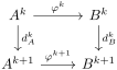
Definition 1.2.4 (Cochain Map).

A cochain map $𝜑 : 𝐴 ∙ \to 𝐵 ∙$ is a collection of linear maps

𝜑 𝑘 : 𝐴 𝑘 ⟶ 𝐵 𝑘

such that for every $𝑘$ ,

𝜑 𝑘 + 1 \circ 𝑑 𝑘 𝐴 = 𝑑 𝑘 𝐵 \circ 𝜑 𝑘 .

That is, the following diagram commutes:

Proposition 1.2.1.

A cochain map $𝜑 : 𝐴 ∙ \to 𝐵 ∙$ induces a linear map on cohomology

𝜑 * : 𝐻 𝑘 (𝐴 ∙) ⟶ 𝐻 𝑘 (𝐵 ∙) .

Definition 1.2.5 (Short Exact Sequence of Cochain Complexes).

A sequence of cochain complexes

0 ⟶ 𝐴 ∙ 𝑖 \to 𝐵 ∙ 𝑗 \to 𝐶 ∙ ⟶ 0

is a short exact sequence of cochain complexes if for every $𝑘$ ,

0 ⟶ 𝐴 𝑘 𝑖 𝑘 ⟶ 𝐵 𝑘 𝑗 𝑘 ⟶ 𝐶 𝑘 ⟶ 0

is a short exact sequence of vector spaces, and $𝑖, 𝑗$ are cochain maps.

1.4 Mayer–Vietoris Sequence

1.4.1 The Zig–Zag Lemma

Theorem 1.3 (Zig–Zag Lemma).

Let

0 ⟶ 𝐴 ∙ 𝑖 \to 𝐵 ∙ 𝑗 \to 𝐶 ∙ ⟶ 0

be a short exact sequence of cochain complexes. Then there is a long exact sequence in cohomology:

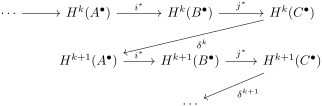
The maps $𝛿 𝑘 : 𝐻 𝑘 (𝐶 ∙) \to 𝐻 𝑘 + 1 (𝐴 ∙)$ are called the connecting homomorphisms. We now describe their construction.

Construction of the Connecting Homomorphism.

Let $[𝑐] \in 𝐻 𝑘 (𝐶 ∙)$ be a cohomology class represented by $𝑐 \in 𝐶 𝑘$ with $𝑑 𝐶 𝑐 = 0$ .

1.

Since $𝑗 𝑘 : 𝐵 𝑘 \to 𝐶 𝑘$ is surjective, there exists $𝑏 \in 𝐵 𝑘$ such that

$𝑗 𝑘 (𝑏) = 𝑐 .$
2.

Since $𝑗$ is a cochain map,

$𝑗 𝑘 + 1 (𝑑 𝐵 𝑏) = 𝑑 𝐶 (𝑗 𝑘 𝑏) = 𝑑 𝐶 𝑐 = 0 .$

By exactness of the rows, there exists a unique $𝑎 \in 𝐴 𝑘 + 1$ such that

$𝑖 𝑘 + 1 (𝑎) = 𝑑 𝐵 𝑏 .$

Uniqueness follows from the injectivity of $𝑖 𝑘 + 1$ .
3.

We show that $𝑎$ is closed:

$𝑖 𝑘 + 2 (𝑑 𝐴 𝑎) = 𝑑 𝐵 (𝑖 𝑘 + 1 (𝑎)) = 𝑑 𝐵 (𝑑 𝐵 𝑏) = 0 .$

Since $𝑖 𝑘 + 2$ is injective, we have $𝑑 𝐴 𝑎 = 0$ . Thus $𝑎$ defines a cohomology class $[𝑎] \in 𝐻 𝑘 + 1 (𝐴 ∙)$ .

We define

𝛿 𝑘 [𝑐] = [𝑎] \in 𝐻 𝑘 + 1 (𝐴 ∙) .

Proposition 1.3.1.

The connecting homomorphism $𝛿 𝑘$ is well-defined, i.e. independent of the choices of $𝑏$ and the representative $𝑐$ .

∎

Proof.

See standard references (e.g., Manifolds §25). The proof is a straightforward diagram chase. ∎

1.4.2 Partitions of Unity

To construct the Mayer–Vietoris sequence for de Rham cohomology, we need a technical tool: partitions of unity.

Definition 1.3.1 (Partition of Unity).

Let $𝑀$ be a smooth manifold, and let ${𝑈 𝛼} 𝛼 \in 𝐴$ be an open cover of $𝑀$ . A $𝐶 \infty$ partition of unity subordinate to ${𝑈 𝛼}$ is a collection of smooth functions

{𝜌 𝛼 : 𝑀 \to ℝ} 𝛼 \in 𝐴

satisfying:

1.

$0 \leq 𝜌 𝛼 (𝑝) \leq 1$ for all $𝑝 \in 𝑀$ and all $𝛼 \in 𝐴$ .
2.

$s u p p 𝜌 𝛼 \subseteq 𝑈 𝛼$ for each $𝛼 \in 𝐴$ .
3.

The collection ${s u p p 𝜌 𝛼} 𝛼 \in 𝐴$ is locally finite: every point $𝑝 \in 𝑀$ has a neighbourhood that intersects only finitely many supports.
4.

For every $𝑝 \in 𝑀$ ,

$\sum 𝛼 \in 𝐴 𝜌 𝛼 (𝑝) = 1 .$

(This sum is finite because of local finiteness.)

Theorem 1.4 (Existence of Partitions of Unity).

Every open cover of a smooth manifold admits a $𝐶 \infty$ partition of unity subordinate to it.

Proof.

See standard references on smooth manifolds (e.g., Manifolds, Appendix C). ∎

1.4.3 The Mayer–Vietoris Theorem

Let $𝑀$ be a smooth manifold, and let ${𝑈, 𝑉}$ be an open cover of $𝑀$ . We will construct a short exact sequence of cochain complexes that induces the Mayer–Vietoris long exact sequence in cohomology.

Define the following maps:

•

The inclusion map

$𝑖 : Ω 𝑘 (𝑀) ⟶ Ω 𝑘 (𝑈) \oplus Ω 𝑘 (𝑉)$

given by

$𝑖 (𝜔) = (𝜔 | 𝑈, 𝜔 | 𝑉) .$
•

The difference map

$𝑗 : Ω 𝑘 (𝑈) \oplus Ω 𝑘 (𝑉) ⟶ Ω 𝑘 (𝑈 \cap 𝑉)$

given by

$𝑗 (𝜔, 𝜏) = 𝜔 | 𝑈 \cap 𝑉 - 𝜏 | 𝑈 \cap 𝑉 .$

Proposition 1.4.1.

The sequence of cochain complexes

0 ⟶ Ω ∙ (𝑀) 𝑖 \to Ω ∙ (𝑈) \oplus Ω ∙ (𝑉) 𝑗 \to Ω ∙ (𝑈 \cap 𝑉) ⟶ 0

is short exact.

Proof.

We verify exactness at each stage.

Exactness at $Ω 𝑘 (𝑀)$ : The map $𝑖$ is injective because if $𝜔 | 𝑈 = 0$ and $𝜔 | 𝑉 = 0$ , then $𝜔 = 0$ on $𝑀 = 𝑈 \cup 𝑉$ .

Exactness at $Ω 𝑘 (𝑈) \oplus Ω 𝑘 (𝑉)$ : Clearly $I m 𝑖 \subseteq k e r 𝑗$ , since

𝑗 (𝑖 (𝜔)) = 𝑗 (𝜔 | 𝑈, 𝜔 | 𝑉) = 𝜔 | 𝑈 \cap 𝑉 - 𝜔 | 𝑈 \cap 𝑉 = 0 .

Conversely, suppose $(𝜔, 𝜏) \in k e r 𝑗$ , so $𝜔 | 𝑈 \cap 𝑉 = 𝜏 | 𝑈 \cap 𝑉$ . We need to find $𝜂 \in Ω 𝑘 (𝑀)$ such that $𝜂 | 𝑈 = 𝜔$ and $𝜂 | 𝑉 = 𝜏$ . This is a gluing problem. Let ${𝜌 𝑈, 𝜌 𝑉}$ be a partition of unity subordinate to the cover ${𝑈, 𝑉}$ . Define

𝜂 = 𝜌 𝑈 𝜔 + 𝜌 𝑉 𝜏,

where $𝜌 𝑈 𝜔$ is extended by zero outside $𝑈$ , and similarly for $𝜌 𝑉 𝜏$ . On $𝑈 \cap 𝑉$ , $𝜔 = 𝜏$ , so

𝜂 | 𝑈 \cap 𝑉 = 𝜌 𝑈 𝜔 + 𝜌 𝑉 𝜔 = 𝜔 .

On $𝑈$ , the term $𝜌 𝑉 𝜏$ is supported in $𝑉 \cap 𝑈$ , and on $𝑉$ , $𝜌 𝑈 𝜔$ is supported in $𝑈 \cap 𝑉$ . Thus $𝜂$ glues properly, and $𝑖 (𝜂) = (𝜔, 𝜏)$ .

Exactness at $Ω 𝑘 (𝑈 \cap 𝑉)$ : The map $𝑗$ is surjective. For any $𝜔 \in Ω 𝑘 (𝑈 \cap 𝑉)$ , we can extend it to a form on $𝑈$ (using a bump function) and take $(𝜔, 0) \in Ω 𝑘 (𝑈) \oplus Ω 𝑘 (𝑉)$ , which satisfies $𝑗 (𝜔, 0) = 𝜔$ . (Alternatively, use a partition of unity to construct the extension.) ∎

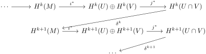
Theorem 1.5 (Mayer–Vietoris Sequence).

Let ${𝑈, 𝑉}$ be an open cover of a smooth manifold $𝑀$ . Then there is a long exact sequence in de Rham cohomology:

Proof.

Apply the Zig–Zag lemma to the short exact sequence of cochain complexes

0 ⟶ Ω ∙ (𝑀) 𝑖 \to Ω ∙ (𝑈) \oplus Ω ∙ (𝑉) 𝑗 \to Ω ∙ (𝑈 \cap 𝑉) ⟶ 0 .

∎

1.4.4 Applications

Example 1.5.1 (Cohomology of Disjoint Unions).

If $𝑀 = 𝐴 ⨿ 𝐵$ is a disjoint union of smooth manifolds, then

𝐻 𝑘 (𝑀) ≅ 𝐻 𝑘 (𝐴) \oplus 𝐻 𝑘 (𝐵) .

This follows directly from the definition of differential forms on a disjoint union.

Example 1.5.2 (Cohomology in Degree 0).

If $𝑀$ has $𝑚$ connected components, then

𝐻 0 (𝑀) ≅ ℝ 𝑚 .

This is because a closed 0-form is a locally constant function, hence constant on each connected component.

Example 1.5.3 (Cohomology of $𝑆 1$ ).

Using the Mayer–Vietoris sequence, we can compute the cohomology of the circle $𝑆 1$ . Let $𝑆 1 = 𝑈 \cup 𝑉$ , where $𝑈$ and $𝑉$ are two open arcs that cover the circle, and $𝑈 \cap 𝑉$ is a disjoint union of two intervals. Since intervals are contractible, $𝐻 𝑘 (𝑈) = 𝐻 𝑘 (𝑉) = 𝐻 𝑘 (𝑈 \cap 𝑉) = 0$ for $𝑘 \geq 1$ , and $𝐻 0$ of each is $ℝ$ . The Mayer–Vietoris sequence gives

0 ⟶ 𝐻 0 (𝑆 1) ⟶ ℝ \oplus ℝ ⟶ ℝ \oplus ℝ ⟶ 𝐻 1 (𝑆 1) ⟶ 0 .

A short computation yields

𝐻 0 (𝑆 1) ≅ ℝ, 𝐻 1 (𝑆 1) ≅ ℝ, 𝐻 𝑘 (𝑆 1) = 0 (𝑘 \geq 2) .

Remark 1.5.1.

The Mayer–Vietoris sequence is an indispensable tool in algebraic topology. It can be used inductively to compute the cohomology of many manifolds by decomposing them into simpler pieces.

1.5 Homotopy Invariance

1.5.1 Homotopy

Definition 1.5.1 (Smooth Homotopy).

Let $𝑀$ and $𝑁$ be smooth manifolds. Two smooth maps

𝑓 0, 𝑓 1 : 𝑀 ⟶ 𝑁

are smoothly homotopic if there exists a smooth map

𝐹 : 𝑀 \times [0, 1] ⟶ 𝑁

such that

𝐹 (𝑥, 0) = 𝑓 0 (𝑥), 𝐹 (𝑥, 1) = 𝑓 1 (𝑥) f o r a l l 𝑥 \in 𝑀 .

The map $𝐹$ is called a smooth homotopy between $𝑓 0$ and $𝑓 1$ . Here “smooth on $𝑀 \times [0, 1]$ ” means that $𝐹$ can be extended to a smooth map on a neighbourhood of $𝑀 \times [0, 1]$ in $𝑀 \times ℝ$ .

Definition 1.5.2 (Homotopy Equivalence).

A smooth map $𝑓 : 𝑀 \to 𝑁$ is a homotopy equivalence if there exists a smooth map $𝑔 : 𝑁 \to 𝑀$ such that

𝑔 \circ 𝑓 \sim i d 𝑀, 𝑓 \circ 𝑔 \sim i d 𝑁 .

The map $𝑔$ is called a homotopy inverse of $𝑓$ . In this case, $𝑀$ and $𝑁$ are said to have the same homotopy type. A manifold with the homotopy type of a point is called contractible.

Example 1.5.4 (Retraction of $ℝ 2 ∖ {0}$ onto $𝑆 1$ ).

Consider the map

𝑟 : ℝ 2 ∖ {0} ⟶ 𝑆 1, 𝑟 (𝑥) = 𝑥 ‖ 𝑥 ‖ .

Let $𝑖 : 𝑆 1 ↪ ℝ 2 ∖ {0}$ be the inclusion. Then

𝑟 \circ 𝑖 = i d 𝑆 1 .

Also,

𝑖 \circ 𝑟 : ℝ 2 ∖ {0} ⟶ ℝ 2 ∖ {0}, (𝑖 \circ 𝑟) (𝑥) = 𝑥 ‖ 𝑥 ‖ .

Define a homotopy

𝐹 : (ℝ 2 ∖ {0}) \times [0, 1] ⟶ ℝ 2 ∖ {0}, 𝐹 (𝑥, 𝑡) = (1 - 𝑡) 𝑥 + 𝑡 𝑥 ‖ 𝑥 ‖ .

Then $𝐹 (𝑥, 0) = 𝑥$ and $𝐹 (𝑥, 1) = 𝑟 (𝑥)$ , so $𝐹$ is a homotopy between $i d ℝ 2 ∖ {0}$ and $𝑖 \circ 𝑟$ . Hence $𝑟$ is a homotopy equivalence, and $ℝ 2 ∖ {0}$ has the homotopy type of $𝑆 1$ .

Definition 1.5.3 (Deformation Retraction).

Let $𝐴 \subset 𝑀$ . A map $𝑟 : 𝑀 \to 𝐴$ is a retraction if $𝑟 | 𝐴 = i d 𝐴$ , i.e. $𝑟 \circ 𝑖 = i d 𝐴$ where $𝑖 : 𝐴 ↪ 𝑀$ is the inclusion. It is a deformation retraction if $𝑖 \circ 𝑟$ is homotopic to $i d 𝑀$ .

Proposition 1.5.1.

A deformation retraction is a homotopy equivalence.

1.5.2 The Homotopy Axiom

Theorem 1.6 (Homotopy Invariance of de Rham Cohomology).

If two smooth maps $𝑓 0, 𝑓 1 : 𝑀 \to 𝑁$ are smoothly homotopic, then they induce the same map on de Rham cohomology:

𝑓 * 0 = 𝑓 * 1 : 𝐻 * (𝑁) ⟶ 𝐻 * (𝑀) .

Proof.

See the next section ∎

Corollary 1.6.1.

If $𝑓 : 𝑀 \to 𝑁$ is a homotopy equivalence, then the induced map

𝑓 * : 𝐻 * (𝑁) ⟶ 𝐻 * (𝑀)

is an isomorphism.

Proof.

Let $𝑔 : 𝑁 \to 𝑀$ be a homotopy inverse of $𝑓$ . Then $𝑔 \circ 𝑓 \sim i d 𝑀$ and $𝑓 \circ 𝑔 \sim i d 𝑁$ . By the homotopy axiom,

(𝑔 \circ 𝑓) * = i d 𝐻 * (𝑀) = 𝑓 * \circ 𝑔 *, (𝑓 \circ 𝑔) * = i d 𝐻 * (𝑁) = 𝑔 * \circ 𝑓 * .

Thus $𝑓 *$ has two-sided inverse $𝑔 *$ , hence is an isomorphism. ∎

Corollary 1.6.2.

Manifolds with the same homotopy type have isomorphic de Rham cohomology.

Example 1.6.1 ( Cohomology of $ℝ 𝑛$ ).

Since $ℝ 𝑛$ is contractible, it has the homotopy type of a point. Hence

𝐻 𝑘 (ℝ 𝑛) ≅ {ℝ, 𝑘 = 0, 0, 𝑘 > 0 .

Example 1.6.2 ( Cohomology of a Cylinder).

The cylinder $𝐶 = 𝑆 1 \times [0, 1]$ deformation retracts onto $𝑆 1$ . Therefore,

𝐻 * (𝐶) ≅ 𝐻 * (𝑆 1) .

In particular, $𝐻 1 (𝐶) ≅ ℝ$ .

1.5.3 The Circle and Its Cohomology

We have already computed $𝐻 * (𝑆 1)$ using Mayer–Vietoris:

𝐻 0 (𝑆 1) ≅ ℝ, 𝐻 1 (𝑆 1) ≅ ℝ, 𝐻 𝑘 (𝑆 1) = 0 (𝑘 \geq 2) .

A generator of $𝐻 1 (𝑆 1)$ can be represented by the angular form

𝜔 = - 𝑦 𝑑 𝑥 + 𝑥 𝑑 𝑦 2 𝜋 (𝑥 2 + 𝑦 2) = 𝑑 𝜃 2 𝜋 .

Indeed,

\int 𝑆 1 𝜔 = 1,

so $[𝜔]$ is the preferred generator.

Remark 1.6.1 (Integration on a Cylinder).

Let $𝐶 = 𝑆 1 \times [0, 1]$ with boundary $𝜕 𝐶 = 𝑆 1 t o p - 𝑆 1 b o t t o m$ . For any closed 1-form $𝜔$ on $𝐶$ , Stokes’ theorem gives

0 = \int 𝐶 𝑑 𝜔 = \int 𝜕 𝐶 𝜔 = \int 𝑆 1 t o p 𝜔 - \int 𝑆 1 b o t t o m 𝜔 .

Thus the integral of a closed 1-form is the same on the top and bottom circles. This fact is used in the construction of the connecting homomorphism in Mayer–Vietoris for the torus.

1.5.4 Cohomology of the Torus

Let $𝑇 = 𝑆 1 \times 𝑆 1$ be the 2-torus. We compute its de Rham cohomology using the Mayer–Vietoris sequence.

Choose an open cover ${𝑈, 𝑉}$ of $𝑇$ as follows. Let $𝑝, 𝑞$ be distinct points on $𝑆 1$ , and set

𝑈 = 𝑆 1 \times (𝑆 1 ∖ {𝑝}), 𝑉 = (𝑆 1 ∖ {𝑞}) \times 𝑆 1 .

Then $𝑈$ and $𝑉$ are each homeomorphic to a cylinder $𝑆 1 \times ℝ$ , so

𝐻 0 (𝑈) ≅ 𝐻 0 (𝑉) ≅ ℝ, 𝐻 1 (𝑈) ≅ 𝐻 1 (𝑉) ≅ ℝ, 𝐻 𝑘 (𝑈) = 𝐻 𝑘 (𝑉) = 0 (𝑘 \geq 2) .

The intersection

𝑈 \cap 𝑉 = (𝑆 1 ∖ {𝑞}) \times (𝑆 1 ∖ {𝑝})

is a disjoint union of two open rectangles (or equivalently, two contractible components), so

𝐻 0 (𝑈 \cap 𝑉) ≅ ℝ \oplus ℝ, 𝐻 1 (𝑈 \cap 𝑉) = 0, 𝐻 𝑘 (𝑈 \cap 𝑉) = 0 (𝑘 \geq 1) .

The Mayer–Vietoris sequence for this cover is:

0 \to 𝐻 0 (𝑇) 𝑖 * ⟶ 𝐻 0 (𝑈) \oplus 𝐻 0 (𝑉) 𝑗 * ⟶ 𝐻 0 (𝑈 \cap 𝑉) 𝛿 0 ⟶ 𝐻 1 (𝑇) 𝑖 * ⟶ 𝐻 1 (𝑈) \oplus 𝐻 1 (𝑉) 𝑗 * ⟶ 𝐻 1 (𝑈 \cap 𝑉) \to 𝐻 2 (𝑇) \to 0 .

Since $𝐻 1 (𝑈 \cap 𝑉) = 0$ , the map $𝑗 * : ℝ \oplus ℝ \to 0$ is zero, so its kernel is all of $ℝ \oplus ℝ$ . Thus $I m 𝑖 * = ℝ 2$ , so $𝑖 * : 𝐻 1 (𝑇) \to ℝ 2$ is surjective. Also, $I m 𝛿 0 = k e r 𝑖 *$ . We compute $𝛿 0$ . The map $𝑗 * : ℝ 2 \to ℝ 2$ (since $𝐻 0 (𝑈 \cap 𝑉) ≅ ℝ 2$ ) sends a pair $(𝛼, 𝛽) \in ℝ 2$ (representing constant functions on U and V) to the pair of restrictions to the two components of $𝑈 \cap 𝑉$ . Actually, the two components of $𝑈 \cap 𝑉$ correspond to the choices of signs; the restriction of a constant function from U and V are identical on each component, so the map is $(𝛼, 𝛽) \mapsto (𝛼 - 𝛽, 𝛼 - 𝛽)$ . Its image is the diagonal ${(𝑡, 𝑡)} \subset ℝ 2$ . Hence $k e r 𝛿 0 = I m 𝑗 * ≅ ℝ$ , so $𝛿 0$ is injective with image of dimension 1. Therefore $k e r 𝑖 *$ is 1-dimensional, and since $𝑖 *$ is surjective onto $ℝ 2$ , we get

𝐻 1 (𝑇) ≅ ℝ 2 .

For $𝐻 2 (𝑇)$ , we need a cover with non-trivial first cohomology of the intersection. A standard choice is to take $𝑈$ and $𝑉$ as two open sets each homeomorphic to a cylinder, but with intersection homeomorphic to two disjoint cylinders, so that $𝐻 1 (𝑈 \cap 𝑉) ≅ ℝ \oplus ℝ$ . With such a cover, the Mayer–Vietoris sequence yields

𝐻 2 (𝑇) ≅ ℝ .

Combining, we obtain

𝐻 0 (𝑇) ≅ ℝ, 𝐻 1 (𝑇) ≅ ℝ 2, 𝐻 2 (𝑇) ≅ ℝ, 𝐻 𝑘 (𝑇) = 0 (𝑘 \geq 3) .

Remark 1.6.2.

The computation of $𝐻 2 (𝑇)$ requires a different choice of open cover (e.g., $𝑈$ and $𝑉$ chosen so that $𝑈 \cap 𝑉$ is two cylinders). The details are standard and can be found in any textbook on differential topology.

Example 1.6.3 (Generators of $𝐻 1 (𝑇)$ ).

On the torus, the two independent 1-forms

𝑑 𝜃 1, 𝑑 𝜃 2

(where $𝜃 𝑖$ are the angular coordinates on each $𝑆 1$ factor) represent a basis of $𝐻 1 (𝑇)$ . Their wedge product $𝑑 𝜃 1 \land 𝑑 𝜃 2$ generates $𝐻 2 (𝑇)$ , and

\int 𝑇 𝑑 𝜃 1 \land 𝑑 𝜃 2 = (2 𝜋) 2 .

Normalizing by $(2 𝜋) - 2$ gives the standard generator with integral 1.

Proof of the Homotopy Axiom

We now give a detailed proof of the homotopy axiom using the language of cochain complexes and chain homotopies.

Definition 1.6.1 (Cochain Homotopy).

Let

𝜑, 𝜓 : 𝐴 ∙ ⟶ 𝐵 ∙

be cochain maps between cochain complexes. A cochain homotopy from $𝜑$ to $𝜓$ is a collection of linear maps

𝐾 : 𝐴 𝑘 ⟶ 𝐵 𝑘 - 1

such that

𝑑 𝐵 \circ 𝐾 + 𝐾 \circ 𝑑 𝐴 = 𝜓 - 𝜑 : 𝐴 𝑘 ⟶ 𝐵 𝑘 .

Lemma 1.6.1.

If there exists a cochain homotopy $𝐾$ from $𝜑$ to $𝜓$ , then

𝜑 * = 𝜓 * : 𝐻 𝑘 (𝐴 ∙) ⟶ 𝐻 𝑘 (𝐵 ∙) .

Proof.

Let $[𝑎] \in 𝐻 𝑘 (𝐴 ∙)$ , so $𝑑 𝐴 𝑎 = 0$ . Then

𝜓 (𝑎) - 𝜑 (𝑎) = 𝑑 𝐵 𝐾 (𝑎) + 𝐾 𝑑 𝐴 (𝑎) = 𝑑 𝐵 𝐾 (𝑎) .

Thus $𝜓 (𝑎) - 𝜑 (𝑎)$ is exact, hence $[𝜓 (𝑎)] = [𝜑 (𝑎)]$ in $𝐻 𝑘 (𝐵 ∙)$ . ∎

Reduction to Two Inclusions

Let $𝐹 : 𝑁 \times [0, 1] \to 𝑀$ be a smooth homotopy between $𝑓 0$ and $𝑓 1$ . Define inclusions

𝑗 0, 𝑗 1 : 𝑁 ⟶ 𝑁 \times [0, 1], 𝑗 0 (𝑥) = (𝑥, 0), 𝑗 1 (𝑥) = (𝑥, 1) .

Then $𝑓 0 = 𝐹 \circ 𝑗 0$ and $𝑓 1 = 𝐹 \circ 𝑗 1$ . By functoriality,

𝑓 * 0 = 𝑗 * 0 \circ 𝐹 *, 𝑓 * 1 = 𝑗 * 1 \circ 𝐹 * .

It suffices to show that

𝑗 * 0 = 𝑗 * 1 : 𝐻 𝑘 (𝑁 \times [0, 1]) ⟶ 𝐻 𝑘 (𝑁) .

We will construct a cochain homotopy $𝐾$ from $𝑗 * 0$ to $𝑗 * 1$ on the de Rham complexes:

𝐾 : Ω 𝑘 (𝑁 \times [0, 1]) ⟶ Ω 𝑘 - 1 (𝑁),

such that

𝑑 𝐾 + 𝐾 𝑑 = 𝑗 * 1 - 𝑗 * 0 .

Local Definition of $𝐾$

On a coordinate chart $(𝑈, 𝑥 1, \dots, 𝑥 𝑛)$ of $𝑁$ , a $𝑘$ -form on $𝑈 \times [0, 1]$ is a sum of two types:

(I) 𝑓 (𝑥, 𝑡) 𝑑 𝑥 𝑖 1 \land \dots \land 𝑑 𝑥 𝑖 𝑘 = : 𝑓 𝑑 𝑥 𝐼,

(I I) 𝑔 (𝑥, 𝑡) 𝑑 𝑡 \land 𝑑 𝑥 𝑗 1 \land \dots \land 𝑑 𝑥 𝑗 𝑘 - 1 = : 𝑔 𝑑 𝑡 \land 𝑑 𝑥 𝐽,

where $𝐼 = (𝑖 1, \dots, 𝑖 𝑘)$ and $𝐽 = (𝑗 1, \dots, 𝑗 𝑘 - 1)$ .

Define $𝐾$ locally by

𝐾 (𝑓 𝑑 𝑥 𝐼) = 0,

𝐾 (𝑔 𝑑 𝑡 \land 𝑑 𝑥 𝐽) = (\int 10 𝑔 (𝑥, 𝑡) 𝑑 𝑡) 𝑑 𝑥 𝐽 .

Verification of the Identity $𝑑 𝐾 + 𝐾 𝑑 = 𝑗 * 1 - 𝑗 * 0$

We verify the identity for forms of type (I). The verification for type (II) is similar and will be omitted.

Type (I): Let $𝜔 = 𝑓 (𝑥, 𝑡) 𝑑 𝑥 𝐼$ . Since $𝐾 (𝜔) = 0$ , we have

(𝑑 𝐾 + 𝐾 𝑑) (𝜔) = 𝐾 (𝑑 𝜔) .

Now

𝑑 𝜔 = 𝑑 𝑓 \land 𝑑 𝑥 𝐼 = 𝑛 \sum 𝑗 = 1 𝜕 𝑓 𝜕 𝑥 𝑗 𝑑 𝑥 𝑗 \land 𝑑 𝑥 𝐼 + 𝜕 𝑓 𝜕 𝑡 𝑑 𝑡 \land 𝑑 𝑥 𝐼 .

The first sum contains no $𝑑 𝑡$ factor, hence its $𝐾$ -image is zero. Therefore

𝐾 (𝑑 𝜔) = 𝐾 (𝜕 𝑓 𝜕 𝑡 𝑑 𝑡 \land 𝑑 𝑥 𝐼) = (\int 10 𝜕 𝑓 𝜕 𝑡 𝑑 𝑡) 𝑑 𝑥 𝐼 = (𝑓 (𝑥, 1) - 𝑓 (𝑥, 0)) 𝑑 𝑥 𝐼 .

On the other hand,

(𝑗 * 1 - 𝑗 * 0) (𝜔) = 𝑓 (𝑥, 1) 𝑑 𝑥 𝐼 - 𝑓 (𝑥, 0) 𝑑 𝑥 𝐼 = (𝑓 (𝑥, 1) - 𝑓 (𝑥, 0)) 𝑑 𝑥 𝐼 .

Thus the identity holds for type (I).

Type (II): A direct computation (reordering the wedge factors so that $𝑑 𝑡$ appears first) shows that

(𝑑 𝐾 + 𝐾 𝑑) (𝑔 𝑑 𝑡 \land 𝑑 𝑥 𝐽) = 0,

while $(𝑗 * 1 - 𝑗 * 0) (𝑔 𝑑 𝑡 \land 𝑑 𝑥 𝐽) = 0$ because the pullback of $𝑑 𝑡$ under $𝑗 0$ and $𝑗 1$ is zero. Hence the identity also holds for type (II).

Coordinate Independence of $𝐾$

We now prove that the local definition of $𝐾$ is independent of the chosen coordinates.

Proposition 1.6.1 (Coordinate Independence of $𝐾$ ).

Let $(𝑈, 𝑥 1, \dots, 𝑥 𝑛)$ and $(𝑉, 𝑦 1, \dots, 𝑦 𝑛)$ be two overlapping coordinate charts on $𝑁$ . For any form $𝜔 \in Ω 𝑘 (𝑁 \times [0, 1])$ , the value of $𝐾 (𝜔)$ computed in the $𝑥$ -coordinates agrees with that computed in the $𝑦$ -coordinates on the intersection $𝑈 \cap 𝑉$ .

Proof.

It suffices to consider forms of type (II), since type (I) is mapped to zero and is trivially coordinate-independent. On the overlap, write

𝜔 = \sum 𝑗 𝑓 𝑗 (𝑥, 𝑡) 𝑑 𝑡 \land 𝑑 𝑥 𝐽 = \sum 𝑖 𝑔 𝑖 (𝑦, 𝑡) 𝑑 𝑡 \land 𝑑 𝑦 𝐼,

where $𝐽 = (𝑗 1, \dots, 𝑗 𝑘 - 1)$ and $𝐼 = (𝑖 1, \dots, 𝑖 𝑘 - 1)$ . The coordinate transformation gives

𝑑 𝑦 𝐼 = \sum 𝐽 𝜕 𝑦 𝐼 𝜕 𝑥 𝐽 𝑑 𝑥 𝐽,

\sum 𝑖 𝑔 𝑖 (𝑦, 𝑡) 𝑑 𝑡 \land 𝑑 𝑦 𝐼 = \sum 𝑖, 𝐽 𝑔 𝑖 (𝑦, 𝑡) 𝜕 𝑦 𝐼 𝜕 𝑥 𝐽 𝑑 𝑡 \land 𝑑 𝑥 𝐽 .

Comparing coefficients with $\sum 𝑗 𝑓 𝑗 (𝑥, 𝑡) 𝑑 𝑡 \land 𝑑 𝑥 𝐽$ , we obtain

𝑓 𝑗 (𝑥, 𝑡) = \sum 𝑖 𝑔 𝑖 (𝑦 (𝑥), 𝑡) 𝜕 𝑦 𝐼 𝜕 𝑥 𝐽 .

Now, in the $𝑥$ -coordinates,

𝐾 𝑥 (𝜔) = \sum 𝑗 (\int 10 𝑓 𝑗 (𝑥, 𝑡) 𝑑 𝑡) 𝑑 𝑥 𝐽,

while in the $𝑦$ -coordinates,

𝐾 𝑦 (𝜔) = \sum 𝑖 (\int 10 𝑔 𝑖 (𝑦, 𝑡) 𝑑 𝑡) 𝑑 𝑦 𝐼 .

Using the relation between $𝑓 𝑗$ and $𝑔 𝑖$ , we have

𝐾 𝑥 (𝜔) = \sum 𝑗 (\int 10 \sum 𝑖 𝑔 𝑖 (𝑦 (𝑥), 𝑡) 𝜕 𝑦 𝐼 𝜕 𝑥 𝐽 𝑑 𝑡) 𝑑 𝑥 𝐽 = \sum 𝑖 (\int 10 𝑔 𝑖 (𝑦 (𝑥), 𝑡) 𝑑 𝑡) \sum 𝐽 𝜕 𝑦 𝐼 𝜕 𝑥 𝐽 𝑑 𝑥 𝐽 = \sum 𝑖 (\int 10 𝑔 𝑖 (𝑦 (𝑥), 𝑡) 𝑑 𝑡) 𝑑 𝑦 𝐼 = 𝐾 𝑦 (𝜔) .

Thus the two expressions agree on $𝑈 \cap 𝑉$ . ∎

The coordinate independence allows us to patch the local definitions of $𝐾$ together using a partition of unity (or simply by defining $𝐾 (𝜔)$ on each chart and gluing). Hence we obtain a global operator

𝐾 : Ω 𝑘 (𝑁 \times [0, 1]) ⟶ Ω 𝑘 - 1 (𝑁) .

Since the identity $𝑑 𝐾 + 𝐾 𝑑 = 𝑗 * 1 - 𝑗 * 0$ is local, and we have verified it on each chart, it holds globally. Therefore $𝐾$ is a cochain homotopy from $𝑗 * 0$ to $𝑗 * 1$ . By the lemma, $𝑗 * 0 = 𝑗 * 1$ on cohomology. Consequently,

𝑓 * 0 = 𝑗 * 0 \circ 𝐹 * = 𝑗 * 1 \circ 𝐹 * = 𝑓 * 1,

which proves the homotopy axiom.

代数拓扑中的微分形式

1 De Rham Cohomology

1.1 Tensors and Forms

1.1.1 Tensors

Definition 1.0.1 (𝑘-tensor).

Example 1.0.1 ( Dual Space).

Definition 1.0.2 (Alternating 𝑘-tensor).

Remark 1.0.1.

Example 1.0.2.

Definition 1.0.3 (Wedge Product).

Example 1.0.3.

Proposition 1.0.1 (Basis of Alternating Tensors).

1.1.2 Differential Forms

Definition 1.0.4 (Differential Form).

Remark 1.0.2.

Definition 1.0.5 (Differential of a Function).

Proposition 1.0.2 ( The expression of k-form in the local coordinate).

Definition 1.0.6 (Smooth Forms).

Theorem 1.1 (Exterior Derivative).

Remark 1.1.1.

Definition 1.1.1 (Closed and Exact Forms).

1.2 The De Rham Cohomology

1.2.1 De Rham Cohomology

Definition 1.1.2 (De Rham Cohomology).

Example 1.1.1 ( Computation of 𝐻∗(ℝ)).

Proposition 1.1.1.

1.2.2 Cohomology with Compact Support

Definition 1.1.3 (Support of a Differential Form).

Definition 1.1.4 (Compact Support Forms).

Proposition 1.1.2 (Support is Decreasing under 𝑑).

Proof.

Corollary 1.1.1.

Definition 1.1.5 (Compact Support Cohomology).

Example 1.1.2 (𝐻∗𝑐(ℝ)).

Remark 1.1.2.

1.3 Diffeomorphism Invariance

1.3.1 Pullback

Definition 1.1.6 (Pullback).

Proposition 1.1.3.

Proof.

Theorem 1.2 (Diffeomorphism Invariance).

Proof.

Example 1.2.1 ( Intervals).

Remark 1.2.1.

1.3.2 Exact Sequences and Cochain Complexes

Definition 1.2.1 (Exact Sequence).

Definition 1.2.2 (Short Exact Sequence).

Remark 1.2.2.

Definition 1.2.3 (Cochain Complex).

Definition 1.2.4 (Cochain Map).

Proposition 1.2.1.

Definition 1.2.5 (Short Exact Sequence of Cochain Complexes).

1.4 Mayer–Vietoris Sequence

1.4.1 The Zig–Zag Lemma

Theorem 1.3 (Zig–Zag Lemma).

Construction of the Connecting Homomorphism.

Proposition 1.3.1.

Proof.

1.4.2 Partitions of Unity

Definition 1.3.1 (Partition of Unity).

Theorem 1.4 (Existence of Partitions of Unity).

Proof.

1.4.3 The Mayer–Vietoris Theorem

Proposition 1.4.1.

Proof.

Theorem 1.5 (Mayer–Vietoris Sequence).

Proof.

1.4.4 Applications

Example 1.5.1 (Cohomology of Disjoint Unions).

Example 1.5.2 (Cohomology in Degree 0).

Example 1.5.3 (Cohomology of 𝑆1).

Remark 1.5.1.

1.5 Homotopy Invariance

1.5.1 Homotopy

Definition 1.5.1 (Smooth Homotopy).

Definition 1.5.2 (Homotopy Equivalence).

Example 1.5.4 (Retraction of ℝ2∖{0} onto 𝑆1).

Definition 1.5.3 (Deformation Retraction).

Proposition 1.5.1.

1.5.2 The Homotopy Axiom

Definition 1.0.1 ( $𝑘$ -tensor).

Definition 1.0.2 (Alternating $𝑘$ -tensor).

Example 1.1.1 ( Computation of $𝐻 * (ℝ)$ ).

Proposition 1.1.2 (Support is Decreasing under $𝑑$ ).

Example 1.1.2 ( $𝐻 * 𝑐 (ℝ)$ ).

Example 1.5.3 (Cohomology of $𝑆 1$ ).

Example 1.5.4 (Retraction of $ℝ 2 ∖ {0}$ onto $𝑆 1$ ).

Example 1.6.1 ( Cohomology of $ℝ 𝑛$ ).

Example 1.6.3 (Generators of $𝐻 1 (𝑇)$ ).

Local Definition of $𝐾$

Verification of the Identity $𝑑 𝐾 + 𝐾 𝑑 = 𝑗 * 1 - 𝑗 * 0$

Coordinate Independence of $𝐾$

Proposition 1.6.1 (Coordinate Independence of $𝐾$ ).